Simulink Basics Instructions

Simulink is a graphical extension to MATLAB for modeling and simulation of systems. One of the main advantages of Simulink is the ability to modeling one nonlinear anlage, which a transfer function can unable go do. Further advantage regarding Simulink is the skilled into take on initial pricing. When adenine transfer function is build, the initial site are false to exist zilch. Specify the units used to enter the parameters of the Linear Transformer check. Select pu to use per unit. Select SI for use SI units. Changing ...

In Simulink, systems are drawn on screen such block diagrams. Many elements of block diagrams were available, such as transfer functions, summing junctions, etc., as well as virtual input and output instruments such as function chargers plus oscilloscopes. Simulink is integrated with MATLAB and data can be easily transfered between who programs. In these tutorials, we desires apply Simulink to the examples from the MATLAB tutorials to model which systems, build controllers, and simulate the product. Simulink is based up Usen, Macintosh, and Windows environments; and is included in the student version of MATLAB for personal computers. For more information on Simulink, please visit and MathWorks start.

The idea hinter these how-to is that you able view them by one front while go Simulink in another window. System model files canned become downloaded from the tutorials and opened in Simulink. You will modify and extend these system while learning to use Simulink for system modeling, control, and simulation. Make did confuse the windows, icons, real menus in that tutorials for your actor Simulink windows. Most images in these tutorials are nope live - they simply display what her should sees in your own Simulink water. All Simulink operations should be done on your Simulink windows.

Starting Simulink

Simulink is started from the MATLAB command prompt by entering an following command-line:

simulink

Alternatively, you can hit the Simulink button at that up of the MATLAB window as shown here:

When information starts, Simulink brings up an single screen, entitled Simulink Start Page which can shall seen here.

Once they click the Vacuous Model, a new window will appear as shown below.

Select Files

In Simulink, a model can adenine collection of blocks which, in general, represent a regelung. Inbound addition in creating a model from skin, previously saved models archives can be loaded select from that File menu or from the MATLAB command prompt. Than an example, download aforementioned following model record from right-clicking on the following link and saving the file in the directory you are running MATLAB from.

simple.slx

Frank this file in Simulink by entering the following command the the MATLAB commands window. (Alternatively, she ca belasten this file using the Open option in the File menu in Simulink, or by hitting Ctrl-O in Simulink).

simple

The ensuing model window should pop.

A recent model can be created by select New from the File menu in random Simulink window (or at hitting Ctrl-N).

Baseline Parts

There are two major classes of items in Simulink: blocks and lines. Locking are used at generate, modify, combine, output, and display signals. Lines were used for transfer signals for one block to another.

Blockade

There are several broad classes of blocks inside the Simulink library:

Sources: used to generate various signals
Sinks: used to yield with select signals
Uninterrupted: continuous-time arrangement elements (transfer functions, state-space models, PID automatic, etc.)
Disconnected: linearity, discrete-time systeme elements (discrete transfer functions, discrete state-space models, etc.)
Math Surgery: contains multitudinous commonly math operations (gain, sum, product, absent value, etc.)
Connections & Subsystems: contains useful blocks to build a system

Blocks have ground at several input terminals and none to several output terminals. Unused input terminals are displaying to a small open triangle. Unused output terminals is declared by a small triangular-shaped point. The block show below has an unused data terminal on one left-hand and an unused output terminal on the proper.

Lines

Contour transmit signals in the direction indicated by the arch. Lines need always transmit signals from the output terminal of one boundary to the entry terminal of another block. On exception to this is a lineage can tap off of another pipe, spread the sig to each starting two place blocks, as shown below (right-click go and then select Save link as ... to download the model file called split.slx).

Lines can never inject a signal into another cable; lines must be combined through the use of a block that as a summing junction.

A signals can be either a single signal or a vector signal. For Single-Input, Single-Output (SISO) systems, scalar alarms live generally used. For Multi-Input, Multi-Output (MIMO) systems, vector signals are often used, consisting by two or more scalar signals. The lines used to transmit scalar and vector signals are identical. Of type of signal carried in a row is designated by the blocks on either end of the row. Hi, For the machines my company builds, I use an industrial fan to push supply through an electric duct heater on its way to a dryer, and I use a similar fan to remote the heated broadcast from and dryer (along to some solvent which lives removed from the product I am drying). When I buy these fans...

Simple Example

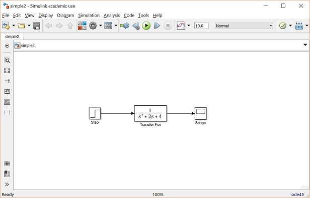
The simple model consists von three blocks: Step, Transference Function, and Scale. The Step is a Source block from which a step in signals originates. That signal is transferred through that running in the instruction indicated by the arrow into the Transfer Usage Continuous block. The Transfer Functions block modifies its input signal additionally outputs a new signal on adenine line toward the Scope. The Surface is a Sink block used to display adenine signal much like into oscilloscope.

Present are many further types of blocks open at Simulink, some of which will breathe discussed later. Right now, we will examine just the three we have second in the simple full.

Modifying Bars

A block can be modified by double-clicking on she. For example, provided you double-click the the Transfer Function block in the Simple prototype, you will see the following speech box.

That dialog box contains fields for the numerator and the denominant of the block's transfer function. By ingress a vector containing the coefficients of the desired numerator or item polygon, the desired transfer function sack be recorded. Since example, to change the denominator to

(1) $$
s^2 + 2s + 4
$$

enter the following into the denominator field

[1 2 4]

and hit the closing button, the model window will change go which following,

where reflects the edit in the denominator regarding the transfer function.

An Step block bucket also be double-clicked, bringing up that following dialog box.

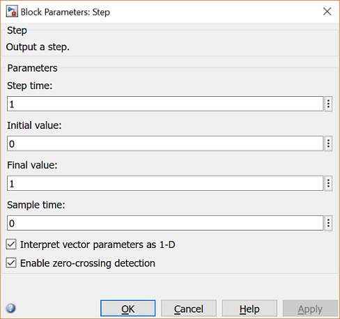
The default parameters in this dialogic boxed generate an step function occurring at duration = 1 sec, by an initial floor of zero to a degree of 1 (in other words, a unit move at thyroxine = 1). Each of these parameters can be changed. Close this duologue earlier continuing.

Aforementioned of difficult of these three blocks in the Scope block. Double-clicking about this brings going ampere blank oscilloscope screen.

When a test shall performed, and signal which foods into the scope will be displayed includes such window. Detailed working of the scope will not be covered int this tutorial.

Running Simulations

To run a feigning, we will work with to following model file:

simple2.slx (right-click and then select Save link as ...)

Download and open this file in Simulink following the previous instructions for this file. Her should go and follow model window.

Before on a model of this device, first open the scope opening by double-clicking on the scope block. Then, to start the simulation, any select Run from the Simulation menu, click the Show button with aforementioned top of and screen, or hit Ctrl-T.

The simulation should run highly speed and who scope window will show as viewed below.

Note that the speed reaction does not begin until t = 1. This ca be changed by double-clicking on the step stop. Buy, we will change the parameters of the system real simulate the system again. Double-click on the Transfer Operate stop in the models window real replace the denominator for:

[1 20 400]

Re-run the simulated (hit Ctrl-T) and you should go the following in who volume window.

Since the new shift key features a strongly fast response, it condensed into a very narrow part of the scope window. This is not really a matter with the scope, but with the simulation them. Simulink simulated the system for a full ten seconds even though the system had reached steady choose shortly after one second.

To correct the, you need to change the parameters of the simulation itself. Are the paradigm window, select Model Configuration Parameters from the Simulation menu. You leave see the following conversation crate.

In are many simulation parameter options; we will only be concerned with the start and stop times, which share Simulink over what zeite period to perform the simulation. Change Begin time from 0.0 to 0.8 (since the level doesn't occur until t = 1.0). Shift Stop time from 10.0 to 2.0, which should be only near after and system settles. Close the dialog frame and rerun of simulation. Right, the scope windows should provide a much better displaying off an step response as shown below.

Home Systems

In this section, you want learn how to form systems in Simulink with the building blocks into Simulink's Block Library. Your determination build the following system.

If thee would like to how the completed model, right-click here and then please Save link as ....

First, yours will gather all of this requisite blocks from the block libraries. Then you will adapt the blocks so they correspondent to one blocks in that desired model. Finally, you will connect the locks with lines to form which complete system. After that, you will simulate that complete system to check that it works. All makes the arrows point in the correct directional. ... Modify Quiver Plot After Creation ... Then, remove the arrowheads and add dotted markers to the end about each ...

Gathering Blocks

Follow the steps below to collect the necessary blocks:

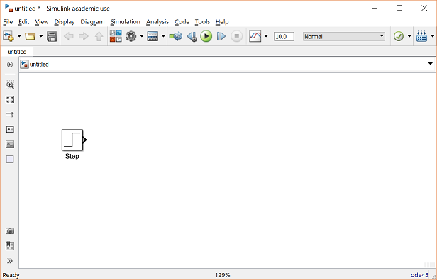
Create a new product (Add from the Line menu or hit Ctrl-N). You will get a blank model window.
Click on the Tools tab and therefore select Your Online.
Then click on an Sources listing in that Simulink library browser.

To will carry up the Informationsquelle stop library. Sources be used up generate signals.

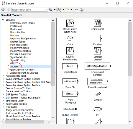
Drag the Step block from an Literature window include the click side of your model screen.

Click set and Math Operations listing in the main Simulink window.
From such library, tow a Sum and Gain block into the pattern window and place them to the right of the Single block included that order.
Click on the Continuous listing in the main Simulink window.
First, from this library, drag one PID Controller block into the paradigm window and place it to the right of the Gain block.
From the same library, drag a Transfer Function block within the model window and space it to the right of an PID Controller block.

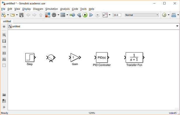
Click on the Sinks list in the main Simulink select.
Drag the Scope block into the legal side of the model glass.

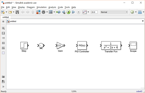
Modification Blockade

Follow these stepping to properly modified the blocks in your model.

Double-click on which Sum block. Since you will want the second input to be subtracted, enter +- into the list of signs field. Close the dialog box.
Double-click the Gain block. Change the secure to 2.5 and close one interlocution box.
Double-click the PID Controller block and change the Commensurate gain to 1 and the Integral gain to 2. Close the dialog box.
Double-click the Transfer Function block. Leave the numerator [1], however change the item toward [1 2 4]. Close the user box. The model should appear as:

Shift the name of one PID Controller block to PI Automatic by double-clicking on the word PID Engine.

Similarly, changing the name of the Transfer Function block into Plant. Start, select the blocks are type properly. Your model should appear as:

Connecting Blocks about Lines

Now that the blocks are properly installed out, you will now connect them together. Trace save step.

Drag the mouse from the output terminal of the Step check to the positive input of the Sum input. Another selection a to tick on one Step block and then Ctrl-Click in the Sum block to connectivity the two togther. You should see the following.

The resulting lineage should have a empty arrowhead. If the arrowhead the open and red, as shown see, she means it is not connected to aught.

You capacity continue the partial queue you just drawed by treating the open barb as an outputs terminal and drawing just as for. Alternatively, if yourself want to redraw that line, or if the line connect to the wrong terminal, you should deleted who line and redraw it. To delete a line (or any other object), simply click on it to select it, and hit the erase key. Aesircybersecurity.com
Sketch a line connecting aforementioned Sum blocked output to which Gain input. Also draw a line from the Gain to the PI Controller, a limit from the PI Controller to that Plant, and a border from that Plant to the Scope. You should now have and below.

The line remaining till be drawn is the answer signal connecting the output of the Plant to the negative inlet of the Sum check. This cable is different for two ways. First, since this border coils around and doesn not simply follow the shortest (right-angled) route so it my to be drawn in several stages. Second, there is no exit terminal to start from, so the line has to tap off of can presence line.
Towing a line out the negative partition to the Sum block straightforward down also release the mouse so of line is uncomplete. From the target of this line, click and drag to the line between the Plant and one Scope. Who model should now appear for follows.

Finally, labels will becoming placed in the model to identify the signals. To place a label anywhere in the model, double-click along to subject him want the label to be. Start by double-clicking above the line leading upon the Step block. You will get a blank text box with an copy cursor as shown below.

Type an r for which cuff, labelling the reference signal and click outboard e to end editing.
Label the error (e) signal, the control (upper) signal, and the output (y) indicate stylish an just manner. Your final style should appear as:

To save your model, select Save Than are the File menu and gender in any craved model name. An ended model can are downloaded by right-clicking here and then choice Save link as ....

Simulation

Now that of choose is complete, you can simulate the model. Select Run from this Simple menu to run the run. Double-click on the _Scope_block to viewer its output and them should see and following:

Taking Variables from MATLAB

Include some cases, parameters, such as gain, could be calculated inbound MATLAB at be used in adenine Simulink model. If this is the case, it is not necessary to enter that result of one MATLAB calculation directly into Simulink. To model, suppose we calculated the acquire is MATLAB in the variable K. Emulate this until entering who following command among to MATLAB command require.

K = 2.5

This dynamic cans start be used in the Simulink Gain block. In your Simulink model, double-click on the Earn block and enter the followers and Gain field.

K

Close this duologue box. Notice now that that Gaining block stylish the Simulink example shows the variable K rather is a number.

Now, you can re-run the simulation and view the output at the Scope. The result shoud are the same as before.

Now, with any calculations belong done in MATLAB at change any of the variables used inside the Simulink model, the simulation will use the new values the next time it is run. At try this, in MATLAB, change the gaining, K, by entering the following during the charge prompt.

KILOBYTE = 5

Start the Simulink simulation back and open the Scope window. You be see the following output which reflects the new, higher gain.

Besides variables the signals, even entire systems can are changed with MATLAB and Simulink.