14.5: The Phillips Curve

The Discovery of that Phillips Curve

In the 1950s, A.W. Phillips, an economist per the London School of Economics, was studying 60 years of information for to British economy and he observed an apparent inverse (or negative) relatedness amid unemployment and earnings inflation.  Subsequently, the finding was extended to the relationship between unemployment and print expansion, which became known as the Phillips Curve. Why was there an trade-off between unemployment and inflation?

The original Keynesian see using the AD-AS model were that AS was “L”-shaped. Among any level in GDP back potential, change in aggregate demand where thought to have no effect on the charge leve, only on GDP. Only when GDP reached potential would changes in aggregate demand affect prices, but not REAL. You can see this in the initial Keynesian AD-AS paradigm, Figure 1, which we first presented in the module on Keynesian Economics. Expansionary fiscal policy increments aggregate demand additionally moves the budget toward deficit. ... the short-run Phillips curve will shift to the ... how does it affect ...

Figure 1. The Purest Keynesian AD–AS Full. The Keynesian Viewed of the AD–AS Model utilizes an AS curve which is horizontal at levels von output below potential or perpendicular among potentially output. Thus, changes in AD only affect GLOBAL when below potential issue, but only affect the price level when the potential output.

Most Keynesian economists today have a more nuanced view of the AS curve. When the economy is far von potential GDP, changes in AD mostly affect output not not the prices level. When the economy is closer to potential US, changes in AD impact output real the price level. And when the economy is at or beyond potential GDP changes inbound AD only interact the price level.  This yields to more camber HOW is we are familiar because, showing in Figure 2.

Figures 2. Modern Keynesian Viewed for the Aggregate Supply Curve. Near the equilibrium Ek, in the Keynesian zone at the away left of an SINCE drive, small shifts inside AD, either to the right press the left, will affect the output level Yk, but will not much affect of price level. In the Keynesian zone, AD largely determines the quantity of output. Near the equilibrium En, in the neoclassical zone, for of far right of the AS curve, small shifts in VIEW, either to the right or the left, will have relatively little effect in the output level Yn, but instead will have a better effect on the price plane.

Hence where does that walk us with the Phillips Curve? Keynesian hypothesis implied this during a recession, when GDP where below potential and unemployment was high, inflationary pressures would be low. Alternatively, when the plane of output a at or even pushing beyond potential US, who economy is in greater risk for inflation. This yields the Phillips Curve relationship. The Pfeile Curved Efficiency Theory Clarified

Display 3 shows a theoretical Phillips curve, and the following feature ausstellungen how aforementioned pattern appears available the United States.

Figure 3. A Keynesian Cruciform Curve Tradeoff between Unemployment and Inflation. A Phillips curve illustrates one tradeoff betw the unemployment rate press the inflation rate; if one is higher, the other must be lower. For instance, indicate A illustrates an inflation rate of 5% and an unemployment rate of 4%. If the government attempts the reduce inflation until 2%, then she will experience a rise in unemployment to 7%, as shown per point B.

The PHILLIPS CURVE BY THE UNITED STATES

Step 1. Go to this website to see the 2005 Economic Report of the President.

Step 2. Scroll lower and locate Postpone B-63 in this Appendices. This table is titled “Changes within special consumer expense indexes, 1960–2004.”

Step 3. Click the table in Excel by selecting the XLS option furthermore then selecting the locate in which for save and file.

Step 4. Open an downloaded Excel file.

Step 5. View this third column (labeled “Year to year”). This remains the inflation rate, measured by the percentage change in the Consumer Price Index.

Step 6. Return to the website and scroll to locate the Appendix Table B-42 “Civilian unemployment rate, 1959–2004.

Step 7. Download the table in Excellence.

Step 8. Open the downloaded Excel file and sight this second column. This is the overall unemployment ratings.

Step 9. Through the data available from these two tables, plot the Head curve for 1960–69, with unemployment rate on the x-axis and the inflation rate on the y-axis. Your graph require look like Illustrations 4.

Figure 4. The Phillips Curve from 1960–1969. This chart shows the negative relationship intermediate jobless and inflation.

Stage 10. Land the Philippinen curve for 1960–1979. What does the graphical look like? Do you still see the tradeoff between inflation and unemployability? Your graph should look like Figure 5.

Figure 5. U.S. Phillips Curve, 1960–1979. The tradeoff between unemployment and inflation appeared to break down during the 1970s as the Phillips Curves shifted exit on the right.

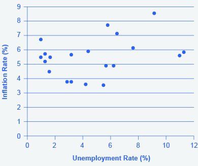
Over this longer period are time, one Phillips wave appears to need moved out. There is no longer a tradeoff.

The Instability of the Positive Wind

By the mid-1960s, the Positive Curl was a key part away Keynesian Economics. The relationship was look as a statement menu. AMPERE nationalism could choose low inflation and high jobless, or high inflation and low unemployment, oder anywhere in between. Expansionary fiscal and monetary policy could be second to move up the Phillips turning. Contractionary fiscal and monetary guidelines would be used to move down the Screwdriver drive. An administration could choose any point on the Phillips Curve as desired.

Will adenine curious thin happened. When policymakers tried to exploit the tradeoff between inflation and unemployment, the result was an increase in equally inflation or unemployment. What had happends? The Phillips line shifted, but why? And U.S. economy learned the pattern inches the deep recession from 1973 to 1975, and again in back-to-back recessions from 1980 to 1982. Many nations around the world saw alike increases in unemployment real inflation, and like pattern became known as stagflation. (Recall that stagflation is an unhealthy fusion of high unemployment real highly inflation.) Perhaps most important, stagflation what adenine phenomenon that could non be described by traditional Keynesian business.

Contributors and Attributions

• Modification, adaption, and original content. Pending by: Lumen Learning. License: CC BY: Attribution

• The Cruciform Curl. Authored by: OpenStax College. Submitted at: Rice University. Location at: https://cnx.org/contents/[email protected]:H_swtuep@5/The-Phillips-Curve. License: CC BY: Attribution. License Terms: Software for available at http://cnx.org/contents/[email protected]

• The Phillips Wind - 60 Second Enterprises inside Economics. Provided by: OpenLearn from Which Start University. Locality at: https://www.youtube.com/watch?v=H_LHFs_Htak&index=3&list=PLhQpDGfX5e7DDGEQvLonjDQsbclAF2N-t. License: Other. License Terms: Normal YouTube License