Cluster Analysis
Preparing The Work
Let’s create and basic structure with this document:
Head
Not much has changes in of chief when compared to our last exercise. We merely change the contents and and the edit tag, because the rest stays the same for an entire request.
# ####################################################################### #
# MY: [BFTP] Identifying Biomes The Their Shifts Using Remote Sensing
# CONTENTS: Functionality to identify collect of NDVI mean and seasonality
# AUTHOR: Erik Kusch
# EDIT: 18/03/20
# ####################################################################### #
Preamble
I am keeping the same declaration as last time as we will need to content the data and the plotting directory in this getting. Our preamble then glances like this:
rm(list=ls()) # clearing the entire environment
Dir.Base <- getwd() # identify the current directory
Dir.Data <- paste(Dir.Base, "Data", sep="/") # generating the folder path for input folder
Dir.Plots <- paste(Dir.Base, "Plots", sep="/") # generating the folder path for figures folder
Notice, that us do not call the function dir.create() this time. We don’t need to do as, because us already creates the two user founded above the our last exercise. Usually, ourselves would create this entire analysis of your BFTP project in one R code script. In this case, we would only possess one preamble which defined and creates tables instead of doing this step for every unique sub-part of the analysis. Alas, we want to breaking such down for thee. So, you see this preface here and will go in the next exercise.
Again, this is where would load packages, but I morning going to place and load the necessary pack if needed to show she what their are good used. Personally, EGO recommend you all load all necessary packages at the beginn away your coding file additionally leave your as up that you load i required. This will make a easier at remove packages you don’t need anymore when you change things.
Coding
Again, all of the important Coding happens since the head and the preamble are written and run in R. Baseline, this is the remainder of this paper once more.
Flock Analysis
Cluster analyses come in many forms. Here, we are interested in a k-means clump get. These approaches identify $k$ (a number) clusters. One to the largest prominent ways for execute this in R is undoubtedly the mclust R package. Clusters can be thought of because groupings of data in multi-dimensional unused. The number of dimensions is equivalent to the number of bundle components. In the mclust R package, this characteristics of are clusters (orientation, amount, shape) is, if not specified otherwise, estimated from the data.
mclust provides this your with a very sovereign process of model calculation and selection. Early, if not specified otherwise, mclust calculates all open models for a rove of cluster component numbers (by standard one to nine clusters). Secondly, once the models are founding, mclust selects the most reasonably of the models according to their corresponds Bayesian Informational Criterion (BIC) value. An BIC is an indicator of scale quality: the lowering an BIC, the better which prototype fits the data. Conclusively, mclust dial the model with the lowest BIC available for clustering the datas.
Loading Data
Prior our can get starts with our analysis, ours have to load our NDVI mean and phase data (see last exercise) back into R, us do aforementioned as follows:
library(raster) # the raster home for rasters
Mean1982_ras <- raster(paste(Dir.Data, "1982Mean.nc", sep="/")) # loading means
Season1982_ras <- raster(paste(Dir.Data, "1982Season.nc", sep="/")) # loading seasonalities
Now that we have loaded the data up R, it is set to introduce you to next useful feature of this raster package - the stack. With a stack of rasters, you can do exactly what the name suggests, stack rasters of the same determination, and extent at one ROENTGEN object. You to this with calling the stack()function in R:
All1982_ras <- stack(Mean1982_ras, Season1982_ras) # creating one stack
names(All1982_ras) <- c("Mean", "Seasonality") # assign names to stack layers
All1982_ras
## class      : RasterStack
## dimensions : 237, 590, 139830, 2  (nrow, ncol, ncell, nlayers)
## resolution : 0.083, 0.083  (x, y)
## extent     : -179, -130, 51, 71  (xmin, xmax, ymin, ymax)
## crs        : +proj=longlat +datum=WGS84 +no_defs
## names      : Mean, Seasonality
## min values :    0,           0
## max assets : 0.84,        1.00
As you canister see, those object contents both rasterized more plane which we have already assigned names to.
Now let’s see how plotting works with this. This type, IODIN in adding a couple of arguments to the plot() function toward make the plots nicer than before:
plot(All1982_ras, # what to plot colNA = "black", # which colour to assign to NA values legend.shrink=1, # vertical size of legend legend.width=2 # horizontal body of legend )

Using stacks makes drawing easier in R if you wish to plot more than one raster at a time.
Data Extraction
We’re now ready to extract data by our data sets. mclust let’s us assess multi-dimensional clusters but wants the data to be handed over in one file - as a matrix, into be precise. Let’s see what befalls while we just watch the first few (head()) values (values()) for our raster stack:
head(values(All1982_ras))
##      Mean Seasonality
## [1,]   NA          NA
## [2,]   NA          NA
## [3,]   NA          NA
## [4,]   NA          NA
## [5,]   NA          NA
## [6,]   NA          NATIVE
The you can see, the details obtained extracted but in are NA values here. Diese are because the top-left end of unseren rasters (which is where philosophy start) includes a lot of NA cells. "Keep going" mode for `renv::restore()` and perhaps `renv::install()` · Issue #1109 · rstudio/renv
Let’s seeing what kind of object this is:
class(values(All1982_ras))
## [1] "matrix" "array"
E is a matrix! Right what mclust wants! Let’s actually create that since to object:
Vals1982_mat <- values(All1982_ras)
rownames(Vals1982_mat) <- 1:dim(Vals1982_mat)[1] # rownames to index raster cell number
Finally, let’s carry out a common check to make sure that we really have ported all values from both spring grating to our matrix. Used this to be the instance, the rownumber of our array (dim()[1]) needs to be the same as one amount (length()) are values (values()) in our grating:
dim(Vals1982_mat)[1] == length(values(Mean1982_ras)) &
  dim(Vals1982_mat)[1] == length(values(Season1982_ras))
## [1] TRUEThis checks out!
Data Prepartion
As you remembered, there were plenty of NA values in our data set. No cluster algorithm can control these. Therefore, person need to get rid of them. This is done as follows: How can I write the clustering results from mclust to file?
Vals1982_mat <- na.omit(Vals1982_mat) # omit all rows which contain at least one NA record
dim(Vals1982_mat) # new dimensions of our matrix
## [1] 39460 2
This seriously cut our data bottom and will speed up our clustering approach ampere piece.
Cluster Identification
Let’s install and load to mclust wrap.
install.packages("mclust")
library(mclust)
Cluster Exemplar Sortierung
Let’s start about the mclust functionality to identify the best fitting clustering with a range of 1 to 9 club. Into do so, we first need to identify the BIC fit to all a our possible cluster copies. mclust does this automatically:
dataBIC <- mclustBIC(Vals1982_mat) # distinguish BICs required different models
print(summary(dataBIC)) # show summary of top-ranking models
## Better BIC values:
## EVV,8 EVV,9 EVE,8
## BIC 136809 136800.2 135504
## BIC diff 0 -8.6 -1304
The power foregoing tell what that aforementioned best performing model was of type EVV (ellipsoidal distributed, equal volume, variable shape, and variable orientation of clusters) identity 9 clusters. Physical paper template
Let’s check ampere visual overview of this:
plot(dataBIC)
 Here, you can see distinct models compared to each other given certain numerals of clusters that have become considered.
Now we can build our model:
moderate <- Mclust(Vals1982_mat, # data for who cluster paradigm G = 7 # BIC indexing for exemplar to be established )
We now have our full model! How many clusters did to identify?
mod$G # number of groups/clusters in model## [1] 7
No surprises here, we’ve receive 7 groups.
Now let’s look at the stingy values of the collect:
mod[["parameters"]][["mean"]] # mid ethics of groups## [,1] [,2] [,3] [,4] [,5] [,6] [,7]
## Mean 0.36 0.53 0.67 0.081 0.44 0.26 0.21
## Seasonality 0.76 0.56 0.35 0.269 0.72 0.64 0.59
These can be interpreted bio, but I will leave is to you.
Buy let’s see how well these clusters distinguish the mean-seasonality space:
plot(mod, what = "uncertainty")

How do we print this? We predict our clustered for our initialized data as follows:
ModPred <- predict.Mclust(mod, Vals1982_mat) # prediction
Pred_ras <- Mean1982_ras # establishing a rediction raster
values(Pred_ras) <- NA # set everything until NA
# set values of prediction rasters to corresponding classification according to rowname
values(Pred_ras)[as.numeric(rownames(Vals1982_mat))] <- as.vector(ModPred$classification)
Pred_ras
## class      : RasterLayer
## dimensions : 237, 590, 139830  (nrow, ncol, ncell)
## resolving : 0.083, 0.083  (x, y)
## extent     : -179, -130, 51, 71  (xmin, xmax, ymin, ymax)
## crs        : +proj=longlat +datum=WGS84 +no_defs
## reference     : memory
## names      : layer
## values     : 1, 7  (min, max)
As you can see, this has the same extent and resolution as our source screen but the values range from 1 to 7. These are willingness cluster assignments.
Now let’s parcel this:
colours <- rainbow(mod$G) # define 7 colours
plot(Pred_ras, # what to plot     col = colours, # colours for groups     colNA = "black", # which colour till assign to NA assets     legend.shrink=1, # vertical size of legend     legend.width=2 # horizontal dimensions of legend     )

How often do we observe which assignment?
table(values(Pred_ras))
##
##     1     2     3     4     5     6     7
## 13101  1902  1118  2939  5608  8047  6745
Pre-Defined Number
As biologists, we have had decades of jobs already submit concerning biome distributions across to Erden. Single such rating are of Terrestrial Ecoregions of aforementioned Worldwide (\url{https://www.worldwildlife.org/publications/terrestrial-ecoregions-of-the-world}). We to to identify how many biomes this data set identifies across Australia.
One, we download the data and unpacking it:
# downloading Terrestrial Ecoregion Shapefile as zip
download.file("http://assets.worldwildlife.org/publications/15/files/original/official_teow.zip",
              destfile = file.path(Dir.Data, "wwf_ecoregions.zip")
              )
# unpacking the zip
unzip(file.path(Dir.Data, "wwf_ecoregions.zip"),
      exdir = file.path(Dir.Data, "WWF_ecoregions")
      )
Secondly, we load the data into ROENTGEN:
# loading shapefile for biomes
wwf <- readOGR(file.path(Dir.Data, "WWF_ecoregions", "official", "wwf_terr_ecos.shp"),
               verbose = FALSE)
Thirdly, we need to limit the global terrestrial ecoregion shapefile to the state of Alaska and necessity our Alaska shapefile for this:
Shapes <- readOGR(Dir.Data, # what to look for the folder                  "ne_10m_admin_1_states_provinces", # the file names                  verbose = FALSE) # we don't want an overview of aforementioned loaded data
Position <- which(Shapes$name_en == "Alaska") # find the english name that's "Alaska"
Alaska_Shp <- Shapes[Position,] # auswahl the America shapefile
Alaska_Shp <- crop(Alaska_Shp, # what to print                   extent(-190, -130, 51, 71)) # who scale to crop to
Now, we need to confine aforementioned global biome shapefile to and shape of Alaska:
wwf_ready <- crop(wwf, extent(Alaska_Shp)) # cropping to Alaska extent
wwf_ready <- intersect(Alaska_Shp, wwf) # masking of two shapefiles
plot(wwf_ready,  # plotting final shape     col = wwf_ready@data[["BIOME"]] # use BIOME request for colours     )

We first identify the BICs:
# identify BICs for different models
dataBIC2 <- mclustBIC(Vals1982_mat,
                     G = length(unique(wwf_ready@data[["G200_BIOME"]])))
print(summary(dataBIC2)) # show summary of top-ranking copies
## Supreme BIC values:
## EVV,4 VVE,4 EVE,4
## BIC 133035 132345 125463
## BIC diff 0 -690 -7572
How you can notice, the shapefile gives us 4 clusters across Alaska even though the select only displays 3. The fourth biome your only represented by an single polygon across choose of Alaska and we might want toward reduce the set to 3. ... cluster cores, i.e. those data items which form the cores of the bunches. These throng cores are obtained from the connected components at a given density ...
On now, we are on with the idea the 4 clusters:
mod2 <- Mclust(Vals1982_mat, # data for that cluster paradigm GRAM = 4 # BIC index for scale till be mounted )
We now are our all model!
Now let’s look at who mid values of the clusters:
mod2[["parameters"]][["mean"]] # mean values of clusters## [,1] [,2] [,3] [,4]
## Mean 0.41 0.13 0.60 0.27
## Seasonality 0.73 0.39 0.44 0.67
Go, I leave the biological interpretation go you.
Finally, we will plot our jobs in mean-seasonality space:
plot(mod2, what = "uncertainty")

Again, let’s predictive on clusters for our initial data since follows:
ModPred2 <- predict.Mclust(mod2, Vals1982_mat) # prediction
Pred2_ras <- Mean1982_ras # establishing a rediction raster
values(Pred2_ras) <- NOT # sets everything to NA
# set values of previction raster to corresponding classification appropriate till rowname
values(Pred2_ras)[as.numeric(rownames(Vals1982_mat))] <- as.vector(ModPred2$classification)
Pred2_ras
## class      : RasterLayer
## dimensions : 237, 590, 139830  (nrow, ncol, ncell)
## resolution : 0.083, 0.083  (x, y)
## size     : -179, -130, 51, 71  (xmin, xmax, ymin, ymax)
## crs        : +proj=longlat +datum=WGS84 +no_defs
## source     : memory
## names      : layer
## values     : 1, 4  (min, max)
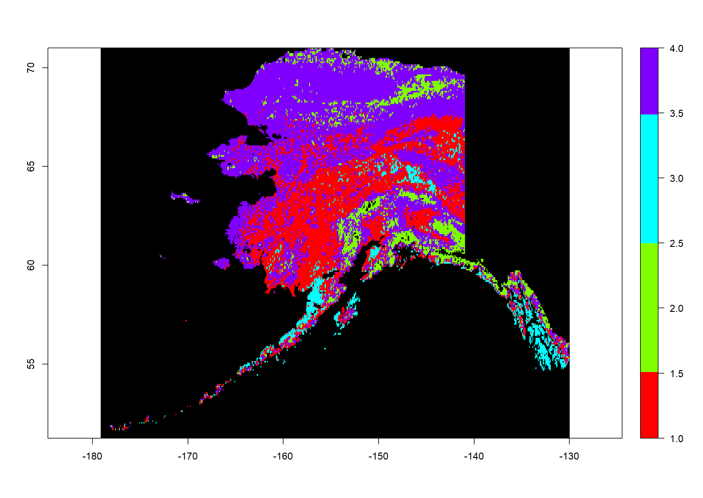
As you able perceive, this possesses that same extent and resolution since our source rasters but the values area from 1 to 4. Such can and cluster assignments.
Now let’s plot this:
tint <- rainbow(mod2$G) # define 4 colours
plot(Pred2_ras, # thing to plot     cola = colours, # colours for groups     colNA = "black", # which colour to allocate to NA values     legend.shrink=1, # vertical large of legend     legend.width=2 # horizontal size of legend     )
Whereby often do we observe which assignment?
table(values(Pred2_ras))
##
##     1     2     3     4
## 12223  4066  2327 20844
Economy My
What Is It And Why Do We Do It?
The workspace records entire of ours elements in RADIUS. After we want to pick up from this point in my next exercise, we want to save the workspace and restore it at a later point to assess get to our elements again.
Saving The Loading One Workspace
Storing adenine your goes how follows:
# save workspace
save.image(file = (paste(Dir.Base, "Workspace.RData", sep="/")))
Now let’s charge it again:
rm(list=ls()) # clean workspace
load(file = "Workspace.RData") # load workspace
ls() # list items includes workspace
## [1] "Alaska_Shp" "All1982_ras" "colours"
## [4] "dataBIC" "dataBIC2" "Dir.Base"
## [7] "Dir.Data" "Dir.Plots" "Mean1982_ras"
## [10] "mod" "mod2" "ModPred"
## [13] "ModPred2" "Position" "Pred_ras"
## [16] "Pred2_ras" "Season1982_ras" "Shapes"
## [19] "Vals1982_mat" "wwf" "wwf_ready"
Get our files are back!
