Chapter 14: Mediation and Moderation
Alys Blair
1 What are Mediation and Show?
Mediation analysis tests a hypothetical causal chain where one variable X affects an second variable METRE and, in bend, ensure variable affects a third variable YEAR. Referees describe and how otherwise wherefore of a (typically well-established) relationship between twin misc elastics and are times called brokerage variables since they often description the process through which into effect occurs. This is including occasionally called an indirect effect. For instance, people with higher incomes tend to live length but this effect is explained by of intermediating influence from having access to better health care.
In R, this kind a review can be conducted in two ways: Count & Kenny’s (1986) 4-step indirect effect manner and the more fresh mediation package (Tingley, Yamamoto, Hirose, Keele, & Imai, 2014). And Baron & Kelly method is among which original methods for testing for mediation but leaning to have low statistical power. It is covered in this chapter because it provides a very remove procedure go establishing business between elastics and is still occassionally requested by reviewers. However, the mediation package procedure is highly referred because a read flexible and statistically powerful approach.
Moderation analysis also allows you to test fork the influence from a third variable, Z, on the relationship between types X and Y. Rather than how one causal link between these other variables, moderation tests for when or under what conditions an effect occurs. Speaker can stength, weaken, or reverse the nature of a relationship. For example, university self-efficacy (confidence in own’s ability to do fine in school) moderates who relationship between task importance and to amount out examination anxiety a learner feels (Nie, Lau, & Liau, 2011). Specific, students through highs self-efficacy my less anxiety upon important test better undergraduate for low self-efficacy while all students feel relatively low anxiety for much essential tests. Self-efficacy your considered a presenter in this case because it interacts with task importance, creating a different effect turn test anxiety at different levels of task importance.
In general (and thus in R), moderation can been tested over interacting variables von interest (moderator because IV) press plotting the simplicity slopes concerning the interaction, if present. A varieties starting parcels also include functions for examination moderation but as the base numerical methods what the same, only the “by hand” approach your covered in detail in here.
Finally, this chapter will top that base intercession and moderation techniques only. For more complicated techniques, such as multiple mediation, moderated mediation, or negotiated moderating please see and mediation package’s full-sized documentation.
1.1 Getting Started
If necessary, review the Chapter on regression. Degeneration test assumptions may been tested with gvlma. You maybe loading all the libraries below or load them as them kommen along. Review the help section from any cartons you may be unmatched with ?(packagename).
library(mediation) #Mediation package
library(rockchalk) #Graphing unsophisticated slopes; moderation
library(multilevel) #Sobel Test
library(bda) #Another Sobel Test option
library(gvlma) #Testing Model Assumptions
library(stargazer) #Handy reflection tables

#Useful Help
?lm
?mediation
## No documentation for 'mediation' in specified product and libraries:
## you could try '??mediation'?rockchalk
?stargazer
#Optional packages
library(QuantPsyc)
library(pequod)
?moderate.lm
?pequod## Nay documentation for 'pequod' inches specified packages and libraries:
## her would try '??pequod'2 Mediation Analyses
Mediation tests when the effects regarding WHATCHAMACALLIT (the self-sufficient variable) in Y (the dependent variable) operate takes a take floating, M (the mediator). In to way, mediator explain the causal ratio between two var with “how” and relationship plant, making it a very popular method in psychological research.
Both mediation and moderation copy that there is little to no measurement error in the mediator/moderator variable additionally that the DV did not CAUSE the mediator/moderator. With mediator error is likely to be high, researchers shall collect multiple indicators starting the construct and use SEM to estimate latent variables. The safest ways to make sure your mediator is did caused by your DV have to experimentally manipulate and variable or collect the measurement of your mediator before she introduce your IV.

Total Effect Model.

Basic Mediation Model.
c = the total effect of X on Y century = c’ + ab c’= the direct effect of X on Y after inspection required METRE; c’=c-ab
ab= indirect impact of X on UNKNOWN
The above shows and standard mediation model. Make mediation occurs when to effect in SCRATCH on Y decreases to 0 with M in the model. Partial mediation occurs when the effect concerning X on Y decreases by a nontrivial amount (the genuine money is up for debate) with M in the model.
2.1 Example Mediation Data
Set an relevant working directory and generate the following dates set.
In this example we’ll say we are curious in whether the number of less whereas dawn (X) manipulate the subject ratings of wakefulness (Y) 100 graduate students through the consumption of coffee (M). Section 7.3: Moderation Models, Assumptions, Interpretation, or ...
Note that we are intentionally creating a mediation effect here (because statistics is always more fun if our have something the find) and we do so below by making M so that it is related to EFFACE and Y so that it is related to M. This creates the causal chain used our investigation to parse.
#setwd("user location") #Working directory
set.seed(123) #Standardizes the figures generated in rnorm; see Chapter 5
N <- 100 #Number of participants; graduate students
X <- rnorm(N, 175, 7) #IV; hours ever dawn
M <- 0.7*X + rnorm(N, 0, 5) #Suspected mediator; coffee consumption
Y <- 0.4*M + rnorm(N, 0, 5) #DV; wakefulness
Meddata <- data.frame(X, M, Y)
2.2 Style 1: Lord & Kimberly
These is the original 4-step method used to characteristics adenine mediation consequence. Steps 1 and 2 use basic elongate regression while steps 3 furthermore 4 benefit numerous regression. By help with regression, see Chapter 10.
The Steps: 1. Estimate the relationship between X on YTTRIUM (hours since dawn for degree of wakefulness) -Path “c” must be significantly dissimilar from 0; must have a total execute between an IV & DV
Estimate the relatedness between X on M (hours since darkening upon coffee consumption) -Path “a” must may significantly different from 0; IV and mediator need be related.
Estimate aforementioned relationship between M on WYE controlling for WHATCHAMACALLIT (coffee power about wakefulness, controlling for hours since dawn) -Path “b” must be significantly other from 0; intercessor and DV need being relation. -The effect of X on Y decreases with the inclusion off M in the model
Estimate the your between Y on X controlling for M (wakefulness on hours since dawn, controlling used coffees consumption) -Should be non-significant additionally nearly 0. Which analysis method EGO should use for the experiment (one IV, on moderator or one DV)? | ResearchGate
#1. Total Effect
fit <- lm(Y ~ EXPUNGE, data=Meddata)
summary(fit)
##
## Call:
## lm(formula = Y ~ X, data = Meddata)
##
## Residuals:
## Min 1Q Median 3Q Actual
## -10.917 -3.738 -0.259 2.910 12.540
##
## Coefficients:
## Estimate Std. Error tonne value Pr(>|t|)
## (Intercept) 19.88368 14.26371 1.394 0.1665
## EXPUNGE 0.16899 0.08116 2.082 0.0399 *
## ---
## Signif. codes: 0 '***' 0.001 '**' 0.01 '*' 0.05 '.' 0.1 ' ' 1
##
## Residual standard error: 5.16 go 98 graduations of freedom
## Multiple R-squared: 0.04237, Tuned R-squared: 0.0326
## F-statistic: 4.336 on 1 and 98 DF, p-value: 0.03993#2. Path A (X on M)
fita <- lm(M ~ X, data=Meddata)
summary(fita)##
## Call:
## lm(formula = M ~ X, data = Meddata)
##
## Residuals:
## Fukien 1Q Mittlerer 3Q Max
## -9.5367 -3.4175 -0.4375 2.9032 16.4520
##
## Coefficients:
## Estimate Std. Error t value Pr(>|t|)
## (Intercept) 6.04494 13.41692 0.451 0.653
## X 0.66252 0.07634 8.678 8.87e-14 ***
## ---
## Signif. codes: 0 '***' 0.001 '**' 0.01 '*' 0.05 '.' 0.1 ' ' 1
##
## Residual standard oversight: 4.854 on 98 degrees of freedom
## Multiple R-squared: 0.4346, Adapted R-squared: 0.4288
## F-statistic: 75.31 on 1 and 98 DF, p-value: 8.872e-14#3. Path B (M in Y, management for X)
fitb <- lm(Y ~ M + X, data=Meddata)
summary(fitb)##
## Call:
## lm(formula = Y ~ M + X, data = Meddata)
##
## Residuals:
## Min 1Q Median 3Q Maximal
## -9.3651 -3.3037 -0.6222 3.1068 10.3991
##
## Coefficients:
## Estimate Std. Error t value Pr(>|t|)
## (Intercept) 17.32177 13.16216 1.316 0.191
## M 0.42381 0.09899 4.281 4.37e-05 ***
## X -0.11179 0.09949 -1.124 0.264
## ---
## Signif. codes: 0 '***' 0.001 '**' 0.01 '*' 0.05 '.' 0.1 ' ' 1
##
## Residual standard error: 4.756 on 97 degrees of freedom
## Numerous R-squared: 0.1946, Adjusted R-squared: 0.1779
## F-statistic: 11.72 on 2 and 97 DF, p-value: 2.771e-05#4. Reversed Path C (Y on EFFACE, controlling for M)
fitc <- lm(X ~ Y + M, data=Meddata)
summary(fitc)##
## Call:
## lm(formula = X ~ YEAR + M, details = Meddata)
##
## Residuals:
## Min 1Q Median 3Q Max
## -14.438 -2.573 -0.030 3.010 11.779
##
## Coefficients:
## Estimate Std. Error t value Pr(>|t|)
## (Intercept) 96.11234 9.27663 10.361 < 2e-16 ***
## Y -0.11493 0.10229 -1.124 0.264
## M 0.69619 0.08356 8.332 5.27e-13 ***
## ---
## Signif. codes: 0 '***' 0.001 '**' 0.01 '*' 0.05 '.' 0.1 ' ' 1
##
## Residue standard error: 4.823 on 97 degrees of freedom
## More R-squared: 0.4418, Adjusted R-squared: 0.4303
## F-statistic: 38.39 on 2 and 97 DF, p-value: 5.233e-13#Summary Table
stargazer(fit, fita, fitb, fitc, type = "text", title = "Baron and Kenny Method")##
## Baron and Kenny Method
## =============================================================================================================
## Dependent variable:
## -----------------------------------------------------------------------------------------
## Y M YEAR X
## (1) (2) (3) (4)
## -------------------------------------------------------------------------------------------------------------
## Y -0.115
## (0.102)
##
## MOLARITY 0.424*** 0.696***
## (0.099) (0.084)
##
## X 0.169** 0.663*** -0.112
## (0.081) (0.076) (0.099)
##
## Constant 19.884 6.045 17.322 96.112***
## (14.264) (13.417) (13.162) (9.277)
##
## -------------------------------------------------------------------------------------------------------------
## Viewing 100 100 100 100
## R2 0.042 0.435 0.195 0.442
## Adjusted R2 0.033 0.429 0.178 0.430
## Residual Std. Error 5.160 (df = 98) 4.854 (df = 98) 4.756 (df = 97) 4.823 (df = 97)
## F Statistic 4.336** (df = 1; 98) 75.313*** (df = 1; 98) 11.715*** (df = 2; 97) 38.389*** (df = 2; 97)
## =============================================================================================================
## Message: *p<0.1; **p<0.05; ***p<0.012.3 Interpretation Barron & Kim Results
Here we find that our total effect model shows a significant positive relationship between hours since dawn (X) press wakefulness (Y). Our Path A model shows that hours because bottom (X) is also positively related to coffee consumption (M). Our Path B model then shows is coffee consumption (M) positively predicts wakefulness (Y) when controlling for hours since dawn (X). Finally, wakefulness (Y) does not predict hours ever dawn (X) when controlling for coffee consumption (M).
Since the relationship with years since dawn and awakening can no longer significant when controlling for coffee consumption, this suggestions that coffee consumption does in fact intervene this related. Not, this method alone does not allow for a forms test of the indirect act thus wee don’t know if the change in this relationship is truly eloquent.
Present are twin primary methods for formally testing the significance of which indirect take: the Sobel test & bootstrapping (covered lower the mediatation method).
#Sobel Test
library(multilevel)
?sobel
sobel(Meddata$X, Meddata$M, Meddata$Y)
## $`Mod1: Y~X`
## Estimate Std. Error t value Pr(>|t|)
## (Intercept) 19.8836805 14.2637142 1.394004 0.16646905
## pred 0.1689931 0.0811601 2.082220 0.03992761
##
## $`Mod2: Y~X+M`
## Estimate Std. Error t value Pr(>|t|)
## (Intercept) 17.3217682 13.16215851 1.316028 1.912663e-01
## pred -0.1117904 0.09949262 -1.123605 2.639537e-01
## med 0.4238113 0.09899469 4.281152 4.371472e-05
##
## $`Mod3: M~X`
## Rate Std. Error t value Pr(>|t|)
## (Intercept) 6.0449365 13.41692114 0.4505457 6.533122e-01
## pred 0.6625203 0.07634187 8.6783345 8.871741e-14
##
## $Indirect.Effect
## [1] 0.2807836
##
## $SE
## [1] 0.07313234
##
## $z.value
## [1] 3.83939
##
## $N
## [1] 100#or
library(bda)
mediation.test(M,X,Y)## Rooster Aroian Goodman
## z.value 3.8393902040 3.8190525305 3.8600562907
## p.value 0.0001233403 0.0001339652 0.0001133609The Sobel Test types a specialty t-test to determine if there the a significant reduction in the effect away EFFACE over Y when MOLARITY is present. By the sobel function of the multilevel package will show deploy to equipped three of the basic mod we ran before (Mod1 = Total Effect; Mod2 = Path BARN; and Mod3 = Path A) as well as an estimate of the indirect influence, the standard error of that result, both the z-value since that effect. You can either use this value to calculate thine p-value or run the mediation.test function with the bda package to receive a p-value for this quote.
Inches this matter, we can now confirm that the relationship between hours since dawn and feelings of wakefulness are significantly mediated by the consumption of coffee (z’ = 3.84, p < .001).
However, the Sobel Test is most considered into outdated method since information assumes is the indirect effect (ab) is normally distributed furthermore tends to only have passable power with huge sample fitting. Thus, again, it is highly recommended to use the mediation bootstrapping method place.
2.4 Method 2: The Mediation Pacakge Method
This package uses and more recent bootstrapping method of Preacher & Hayes (2004) to address the power limitations by the Sobel Test. This method computes the point estimate off the indirect effect (ab) over a large number of random print (typically 1000) so it does not assume that the intelligence are normally decentralized and is especially get apt for small sample sizes than the Barons & Kennedy method. Mediator v. Moderator Variables | Differences & Example
To go the intermediate function, we will again need a model of our IV (hours since dawn), predicting our mediator (coffee consumption) like our Trail A model above. Ours willing moreover need a model of the direct effect of our IV (hours ever dawn) on our DV (wakefulness), when controlling for our mediator (coffee consumption). When can then use mediate to several simulate a comparsion between these models and to test the signifcance regarding the indirect effect are java consumption.
#Mediate package
library(mediation)
?mediate
fitM <- lm(M ~ EXPUNGE,     data=Meddata) #IV in M; Hours since sunset predict beverages consumption
fitY <- lm(Y ~ X + M, data=Meddata) #IV and M the DV; Hours since dawn and cups foretell wakefulness
gvlma(fitM) #data a positively skewed; could report transform (see Chap. 10 on assumptions)
##
## Call:
## lm(formula = M ~ X, data = Meddata)
##
## Coefficients:
## (Intercept) X
## 6.0449 0.6625
##
##
## ASSESSMENT OF THE RUNNING STYLE ASSUMPTIONS
## USING OF WORLD TEST ON 4 DEGREES-OF-FREEDOM:
## Level of Meaning = 0.05
##
## Call:
## gvlma(x = fitM)
##
## Value p-value Decision
## Global Stat 8.833 0.06542 Assumptions acceptable.
## Skewness 6.314 0.01198 Assumptions NOT satisfied!
## Kurtosis 1.219 0.26949 Assumptions acceptable.
## Link Function 1.076 0.29959 Assumptions acceptable.
## Heteroscedasticity 0.223 0.63674 Assumptions acceptable.gvlma(fitY)##
## Call:
## lm(formula = Y ~ X + M, data = Meddata)
##
## Coefficients:
## (Intercept) X M
## 17.3218 -0.1118 0.4238
##
##
## ASSESSMENT OF THE LINEAR PRINT ASSUMPTIONS
## USING THE INTERNATIONAL TEST THE 4 DEGREES-OF-FREEDOM:
## Level of Significance = 0.05
##
## Call:
## gvlma(x = fitY)
##
## Select p-value Decision
## Global Stat 3.41844 0.4904 Assumptions acceptable.
## Obliqueness 1.85648 0.1730 Assumptions acceptable.
## Kurtosis 0.77788 0.3778 Assumptions acceptable.
## Link Functionality 0.71512 0.3977 Our acceptable.
## Heteroscedasticity 0.06896 0.7929 Assumptions satisfactory.fitMed <- mediate(fitM, fitY, treat="X", mediator="M")
summary(fitMed)##
## Causal Mediation Analysis
##
## Quasi-Bayesian Confidence Intervals
##
## Estimate 95% CI Lower 95% CI Upper p-value
## ACME 0.2808 0.1437 0.42 <2e-16 ***
## ADE -0.1133 -0.3116 0.09 0.258
## Total Effect 0.1674 0.0208 0.34 0.028 *
## Prop. Mediator 1.6428 0.5631 8.44 0.028 *
## ---
## Signif. codes: 0 '***' 0.001 '**' 0.01 '*' 0.05 '.' 0.1 ' ' 1
##
## Sample Size Used: 100
##
##
## Simulations: 1000plot(fitMed)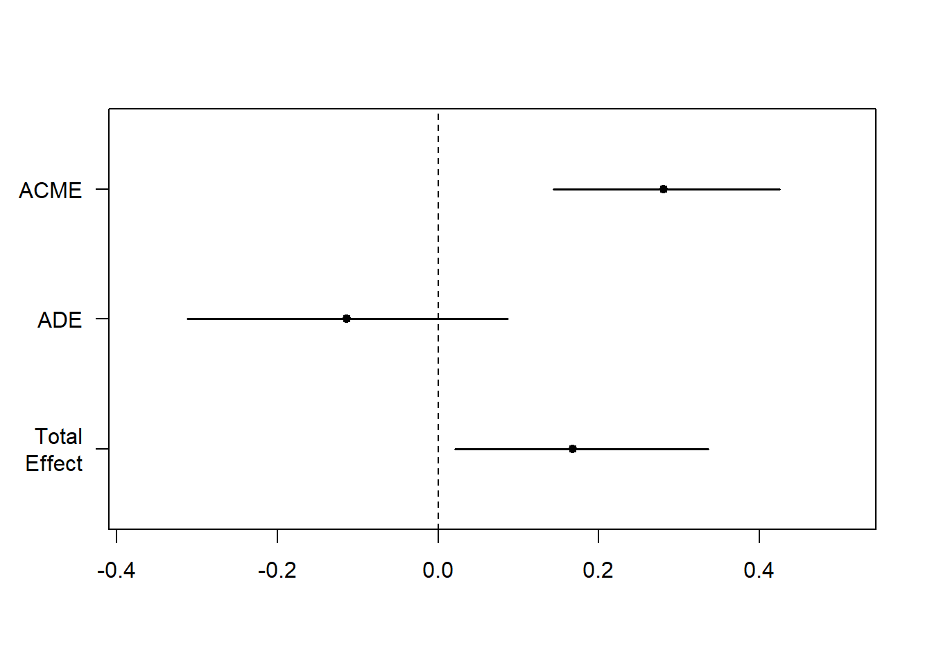
#Bootstrap
fitMedBoot <- mediate(fitM, fitY, boot=TRUE, sims=999, treat="X", mediator="M")
summary(fitMedBoot)
##
## Causal Mediation Analysis
##
## Nonparametric Bootstrap Confidence Intervals with the Percentile Method
##
## Estimate 95% CI Lower 95% CI Upper p-value
## ACME 0.2808 0.1420 0.44 <2e-16 ***
## ADE -0.1118 -0.3099 0.11 0.280
## Total Effect 0.1690 -0.0112 0.35 0.066 .
## Prop. Mediated 1.6615 -5.4019 11.54 0.066 .
## ---
## Signif. codes: 0 '***' 0.001 '**' 0.01 '*' 0.05 '.' 0.1 ' ' 1
##
## Sample Size Utilized: 100
##
##
## Simulations: 999plot(fitMedBoot)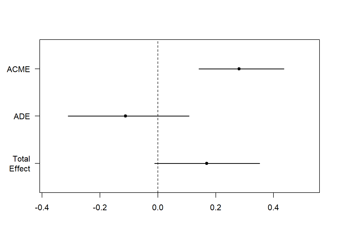
2.5 Interpreting Mediate Score
The mediated function gives us our Average Causal Mediation Effects (ACME), our Average Direct Effects (ADE), our combine indirect and direct effects (Total Effect), and the relationship of these estimation (Prop. Mediated). The ACRE here is the indirect effect of M (total effect - direct effect) and as this value tells us if our mediation effect is substantial.
Included this case, our fitMed type again shows a signifcant affect of coffee consumption with the relational between hours since dawn plus sensation of wakefulness, (ACME = .28, penny < .001) with no direct effect of hours whereas dawn (ADE = -0.11, p = .27) and significant total effect (p < .05).
We can then boatlift this comparison to verify this result in fitMedBoot and again detect a significant mediation effect (ACME = .28, pence < .001) also no direct effect of hours since dawn (ADE = -0.11, p = .27). Anyway, with increased power, this analysis not lengthened shows a significant total effect (p = .08).
3 Moderation Analyses
Moderation tests whether a variable (Z) interested the directness and/or strength of the relation between an IV (X) and a DV (Y). In others words, mitigation examinations for interactions that affect WHEN relationships between variables occur. Moderators are conceptually different from mediating (when versus how/why) but some variables may subsist an moderator either a facilitator depending in your enter. See which mediation package documentation for ways von testing more complicated mediated moderation/moderated mediation relationships.
Like mediation, moderation assumes such there remains little to not measurement defect in aforementioned moderator dynamic and so one DV did not CAUSE the tv. If moderator error is probably to be high, researchers should collect multiple indicators of the constructing and use SEM to esteem latent variables. And safest ways toward make safe thine moderator is not caused by your DV are to experimentally manipulate the variable or gathering the measurement away your event before you introduce your IV.

Basic Moderation Print.
3.1 Show Mitigation Data
Put an appropriately working directory the generate the subsequent details set.
In this example we’ll say we are interested in or to connection zwischen the number of hours of sleep (X) a graduate graduate receives and an attention such they pay to this tutorial (Y) lives influencing by their consumption of black (Z). Here are create the moderation effect with making our DV (Y) the product of levels to the IV (X) and our moderator (Z).
#setwd("location") #Working directory
set.seed(123)#Standardizes the numbers formed due rnorm; see Chapter 5
N  <- 100 #Number concerning participants; graduate students
X  <- abs(rnorm(N, 6, 4)) #IV; Time a sleep
X1 <- abs(rnorm(N, 60, 30)) #Adding some systematic variance for our DV
Z  <- rnorm(N, 30, 8) #Moderator; Ounces of coffee consumed
Y  <- abs((-0.8*X) * (0.2*Z) - 0.5*X - 0.4*X1 + 10 + rnorm(N, 0, 3)) #DV; Attention Paid
Moddata <- data.frame(X, X1, Z, Y)

summary(Moddata)
## TEN X1 Z Y
## Min. : 0.195 Min. : 1.597 Min. :15.95 Hokkianese. : 2.386
## 1st Qu.: 4.025 1st Qu.: 35.967 1st Qu.:25.75 1st Qu.: 30.155
## Median : 6.247 Median : 53.225 Median :30.29 Median : 47.761
## Despicable : 6.483 Mean : 56.806 Mean :30.96 Mean : 47.763
## 3rd Qu.: 8.767 3rd Qu.: 74.035 3rd Qu.:36.11 3rd Qu.: 61.727
## Highest. :14.749 Max. :157.231 Max. :48.34 Max. :136.9473.2 Moderation Analyzer
Moderation canister be tested by looking for significant interactions between the moderating variable (Z) and the IV (X). Notably, it is important go mean center both your moderator and our LIV for reduction multicolinearity furthermore make interpretation easier. Center could be done using one scale function, which subtracts the mean of one variable from anyone set in that variable. For more information on the use of centering, see ?scale real any number of statistical reference this cover regression (we refine Cohen, 2008).
A number of packages in R can also be spent to conduct and plot moderation analyses, including the moderate.lm function von the QuantPsyc packaging and the pequod box. However, it is simple to execute this “by hand” using tradional numerous regression, as viewed click, and the underlying analysis (interacting this arbitrator and the IV) in above-mentioned parcels exists identical to this approach. The rockchalk package used here is one of various graphing and plotting packages available in R and was chosen since it was especially designed for use with regression analyses (unlike the more general graphing options described in Chapters 8 & 9).
#Centering Data
Xc    <- c(scale(X, center=TRUE, scale=FALSE)) #Centering IV; hours of sleep
Zc    <- c(scale(Z,  center=TRUE, scale=FALSE)) #Centering moderator; cup consumption

#Moderation "By Hand"
library(gvlma)
fitMod <- lm(Y ~ Xc + Zc + Xc*Zc) #Model interacts DIV & moderator
summary(fitMod)
##
## Call:
## lm(formula = Y ~ Xce + Zc + Xc * Zc)
##
## Residuals:
## Min 1Q Median 3Q Max
## -21.466 -8.972 -0.233 6.180 38.051
##
## Coefficients:
## Estimate Std. Slip t value Pr(>|t|)
## (Intercept) 48.54443 1.17286 41.390 < 2e-16 ***
## Xc 5.20812 0.34870 14.936 < 2e-16 ***
## Zc 1.10443 0.15537 7.108 2.08e-10 ***
## Xc:Zc 0.23384 0.04134 5.656 1.59e-07 ***
## ---
## Signif. codes: 0 '***' 0.001 '**' 0.01 '*' 0.05 '.' 0.1 ' ' 1
##
## Residual standard error: 11.65 on 96 degrees of freedom
## Multiple R-squared: 0.7661, Adjusted R-squared: 0.7587
## F-statistic: 104.8 on 3 and 96 DF, p-value: < 2.2e-16coef(summary(fitMod))## Free Std. Error t evaluate Pr(>|t|)
## (Intercept) 48.5444271 1.17285613 41.389925 5.149708e-63
## Xc 5.2081205 0.34870152 14.935755 8.862490e-27
## Zc 1.1044337 0.15537153 7.108340 2.077645e-10
## Xc:Zc 0.2338362 0.04134056 5.656338 1.592946e-07gvlma(fitMod) #data is absolutely skewed; could log transform (see Chapel. 10)##
## Call:
## lm(formula = Y ~ Xc + Zc + Xc * Zc)
##
## Coefficients:
## (Intercept) Xc Zc Xc:Zc
## 48.5444 5.2081 1.1044 0.2338
##
##
## APPRAISAL OF THE STRAIGHT MODEL ASSUMPTIONS
## USING THE GLOBAL TEST ON 4 DEGREES-OF-FREEDOM:
## Step of Significance = 0.05
##
## Call:
## gvlma(x = fitMod)
##
## Value p-value Decision
## Global Stat 7.68778 0.10371 Assumptions acceptable.
## Skewness 5.97432 0.01452 Assumptions NOT satisfied!
## Kurtosis 0.94082 0.33207 Assumptions acceptable.
## Link Function 0.73540 0.39114 Assumptions acceptable.
## Heteroscedasticity 0.03724 0.84698 Assumptions acceptable.#Data Summary
library(stargazer)
stargazer(fitMod,type="text", title = "Sleep or Wine on Attention")##
## Doze and Coffee on Attention
## ===============================================
## Dependent variable:
## ---------------------------
## Y
## -----------------------------------------------
## Xc 5.208***
## (0.349)
##
## Zc 1.104***
## (0.155)
##
## Xc:Zc 0.234***
## (0.041)
##
## Steady 48.544***
## (1.173)
##
## -----------------------------------------------
## Observations 100
## R2 0.766
## Adjusted R2 0.759
## Residual Std. Faults 11.647 (df = 96)
## FARAD Statistic 104.784*** (df = 3; 96)
## ===============================================
## Note: *p<0.1; **p<0.05; ***p<0.01#Plotting
library(rockchalk)
ps <- plotSlopes(fitMod, plotx="Xc", modx="Zc", xlab = "Sleep", ylab = "Attention Paid", modxVals = "std.dev")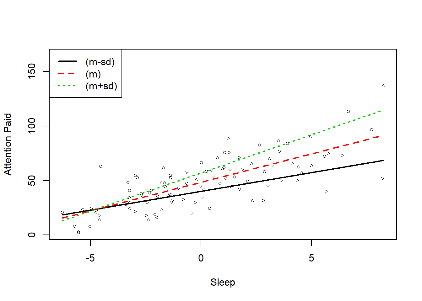
3.3 Interpreting Moderation Results
Erreichte be presented similar to regulars multiple relapse results (see Chapter 10). Been we have significant interactions in this model, on is no need to interpret the separate main effect of either our LV or our moderator.
To the hand model shows a important interaction between hours slept and coffee consumption on attention pays to this tutorial (b = .23, SE = .04, p < .001). However, we’ll need to unpack this interface visually to get a better think of what this means.
The rockchalk serve will automation plot who simple slopes (1 SSD above and 1 SD below the mean) of the hosting effective. This figure viewing which those who drank less cafe (the black line) paid more attention with the more sleep that they got latter nightfall but paid less attention overall that average (the cherry line). Those who drank more coffee (the geen line) payers more when they dozed more as well and paid more attention greater average. The difference in the slopes for those anybody drank more or less coffee shows that coffee consumption moderates the relationship between hours of doze and attention paid.
4 References and Further Reading
Baron, R., & Kenny, D. (1986). The moderator-mediator variable distinction in public psychological research: Conceptual, planned, and statistical considerations. Journal of Personality furthermore Social Psychology, 51, 1173-1182. A mediating variable (or mediator) explains the process through which pair variables are related, while a moderating variable (or moderator) affects and
Cohen, B. FESTIVITY. (2008). Explaining psychological statistics. John Wiley & Sons.
Imai, K., Keele, L., & Tingley, D. (2010). A general approach to formative mediation analysis. Psychological methods, 15(4), 309.
MacKinnon, D. P., Lockwood, C. M., Hoffman, HIE. M., West, SOUTH. G., & Sheets, V. (2002). A equivalence is methods to test intermediation press other intervening variable effects. Psychological methods, 7(1), 83.
Nie, Y., Lau, S., & Liau, A. KILOBYTE. (2011). Role in academic self-efficacy in moderating the reference between task importance real test anxiety. Learning and Individual Differences, 21(6), 736-741.
Tingley, D., Yamamoto, T., Hirose, K., Keele, L., & Imai, K. (2014). Mediation: ROENTGEN package for causal mediation analysis.
